TL;DR: Connect a keyboard-emulation barcode scanner, build a Master Inventory tab and a Stock Log tab, and let XLOOKUP name the product the moment you scan it. A SUMIFS column then recalculates on-hand stock from every logged IN and OUT. Setup takes about 30 minutes, or you can start from the finished workbook. The only unavoidable cost is the scanner — roughly $25–50 — because Google Sheets and Excel for the web are free.
- This is semi-automated, not hands-free. The scanner types the barcode; you still supply the timestamp, IN/OUT, and quantity.
- Format both barcode columns as Text before you scan anything. A Text/Number mismatch between the two tabs makes
XLOOKUPfail on barcodes that plainly exist. XLOOKUPneeds Microsoft 365, Excel 2021, or Excel 2024. Excel 2016 and 2019 do not have it — use theVLOOKUPvariant below.- Never timestamp with
NOW(). It rewrites every past entry the next time the workbook recalculates.
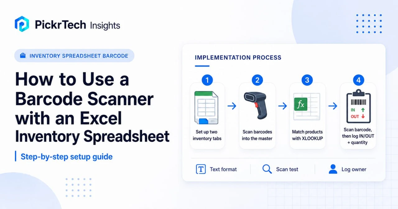
What you need before the first scan
Manual barcode entry creates an avoidable error point: a mistyped digit can produce an unknown code or, less commonly, match the wrong item if that code already exists. A scanner removes that keystroke without requiring a database or an inventory-software subscription. Three things have to be in place first.
- A spreadsheet with
XLOOKUP: Microsoft 365, Excel 2021, or Excel 2024. Microsoft states that XLOOKUP is not available in Excel 2016 or Excel 2019 — on those versions use theVLOOKUPvariant in the templates section. Google Sheets also supportsXLOOKUPand the formulas used here. The menu paths and screenshots below follow desktop Excel; Google Sheets uses different menus for data validation, conditional formatting, frozen rows, and sheet protection. - A scanner in HID / keyboard-emulation mode, USB or Bluetooth. A 1D scanner covers UPC, EAN, and Code 128. Choose a 2D imager only if your labels are QR codes — a 1D-only unit will never read them. A Bluetooth scanner in HID mode feeds the spreadsheet the same way a wired one does, but pairing, battery behavior, and keyboard layout vary by model, so test it in a blank text field first.
- Physical labels on your products: existing UPC/EAN for retail goods, or your own Code 128 item IDs for internal tracking. For products sold through retail or marketplace channels that require a GTIN, use a properly assigned identifier from GS1 rather than inventing a UPC or EAN number.
Before you buy the scanner, confirm two things on the product page: that it supports USB HID or keyboard-emulation mode, and that it can be configured to send an Enter (carriage return) suffix after each scan. Without the Enter suffix, you lose the automatic row advance this workflow depends on.
One person should own the Master Inventory tab and build the workbook. Stockroom or retail staff run the scanner and only ever touch the Stock Log.
Estimated time: about 30 minutes to build, plus however long your initial catalog scan takes
Difficulty: Beginner
Build the workbook: two tabs, one lookup, one running total
Step 1: Set up your two tabs
The structural decision that matters most is keeping the product database physically separate from the transaction log. Open a blank workbook and create two working tabs: Master Inventory and Stock Log. To match the example workbook and screenshots in this guide, use Row 1 for a sheet title, Row 2 for column headers, and start your data in Row 3. During a fast scanning session it is easy to overwrite a row; separating product definitions from movement records limits the damage of a bad paste or scan session.
Master Inventory, Row 2:
- A2: Barcode
- B2: Product Name
- C2: Starting Quantity
- D2: Reorder Point
- E2: Current Stock (the formula starts in E3 in Step 5)
Stock Log, Row 2:
- A2: Timestamp
- B2: Barcode Scanned
- C2: Product Name (the formula starts in C3 in Step 4)
- D2: Movement Type (IN or OUT)
- E2: Quantity
The Reorder Point in column D is a number you supply, not one the workbook derives. If you have not calculated it from your own usage and supplier lead times, the inventory process worksheet works through that calculation before you fill this column in.
Now format both barcode columns as Text before scanning. Excel can display long numeric codes in scientific notation, but the display format alone does not mean the stored value has changed. The real risks are different: numeric entry removes leading zeros, and Excel preserves only the first 15 digits of a number. Storing barcodes as Text keeps the identifier exactly as entered and also prevents a Text/Number mismatch between the master and log lookup columns.
If you already scanned codes before changing the format, inspect the original labels. A code that lost a leading zero or exceeded Excel’s numeric precision should be scanned again after the column is formatted as Text; changing the format does not reconstruct digits that were already altered.
Expected outcome: A workbook with a dedicated master database and an active log, both storing barcodes as text.
Step 2: Connect the scanner and prove it works
Plug the scanner into a USB port and wait for the operating system to recognize it. Most scanners are “keyboard wedge” devices: the computer treats them as an ordinary keyboard, so there is no driver to install and no software to configure.
Open Notepad or any blank text field and scan a physical item. You should see the digits appear instantly, followed by a line break. If the digits appear but the cursor stays on the same line, the Enter suffix is not enabled — find the configuration barcode in the scanner’s manual and scan it to switch the suffix on. Do this now, in Notepad, rather than discovering it halfway through your first catalog session.
Expected outcome: A scan types the barcode digits and presses Enter, with no software in between.
Step 3: Build the product database
The Master Inventory tab is the source of truth for everything that follows, so it is worth the time to get it right. Click cell A3 and scan your first product. The barcode lands in A3 and the cursor drops to A4. Move across to B3 for the product name, C3 for starting quantity, and D3 for the reorder point.
Repeat for every unique item. With a few hundred SKUs this goes much faster in pairs — one person scans down column A while the other types names into column B afterwards.
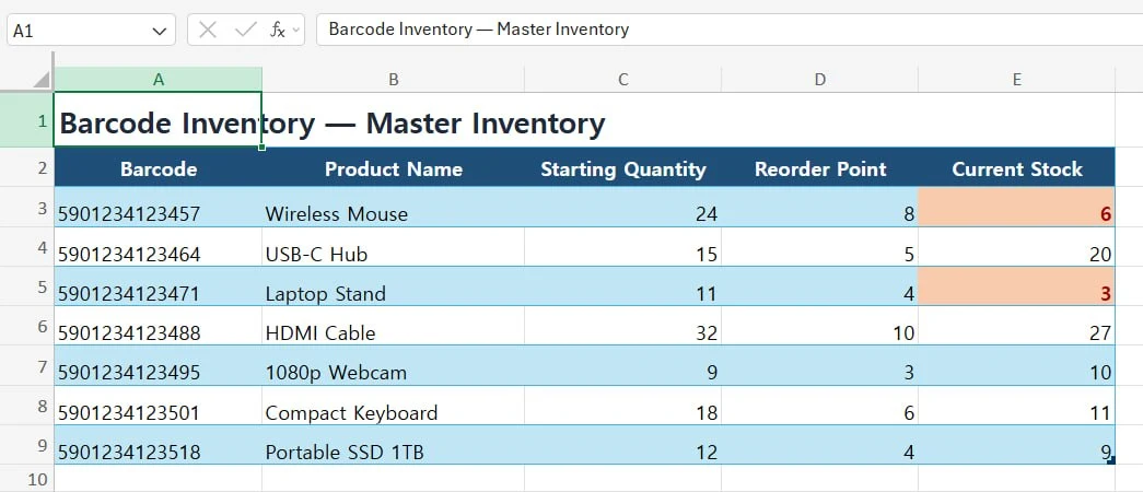
One rule: a barcode should map to one product definition. Do not use Remove Duplicates as the first cleanup step on the master, because Excel removes duplicate records rather than asking which product row is correct. Instead, select the barcode range and go to Home > Conditional Formatting > Highlight Cells Rules > Duplicate Values. Review every highlighted barcode, decide which product row is correct, and then correct or delete the bad record manually.
Expected outcome: A reviewed list of every item you carry, with one product definition per barcode plus starting stock and a reorder threshold.
Step 4: Log stock IN and OUT
Be clear about what this step is and is not. The scanner removes the barcode typing and Excel identifies the product automatically. It does not know whether the box in your hand is arriving or leaving, or how many units are in it. Those two fields, plus the timestamp, stay manual.
On the Stock Log tab, click C3 and enter:
=IF(B3="", "", XLOOKUP(B3, 'Master Inventory'!A:A, 'Master Inventory'!B:B, "Unknown Product"))
That fourth XLOOKUP argument does the job of the IFERROR wrapper you may know from VLOOKUP: an unrecognized barcode shows “Unknown Product” rather than an error. The outer IF keeps empty rows blank, which matters more than it looks — without it, every unused row below your data reads “Unknown Product”, and staff quickly learn to ignore the exact message that is supposed to stop them. Drag the formula down. On Excel 2016 or 2019, use the VLOOKUP version from the templates section below.
Now scan a product into B3. The barcode lands, Enter fires, the cursor drops to B4 — and C3 fills in with the product name from your master sheet. That instant confirmation is the whole payoff: if C3 says “Unknown Product”, you know immediately that the item is missing from the master, and you can fix it before the count is wrong.
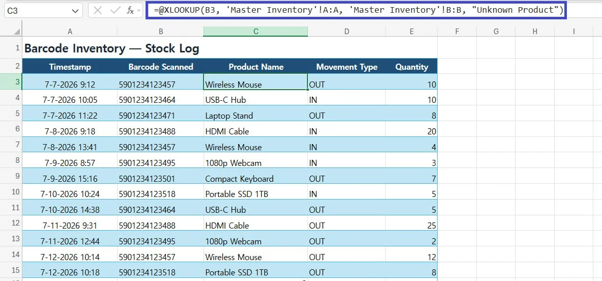
In column D, record IN for received stock and returns, or OUT for anything sold or shipped. Do not leave this to typing. Select D3 down, go to Data > Data Validation, choose List, and enter IN,OUT as the source. The SUMIFS formula in the next step matches on these exact strings, so a stray “in ” with a trailing space silently drops that movement out of the count. A dropdown removes the possibility entirely. Enter the quantity moved in column E.
Finally, the timestamp in column A. In Excel on Windows, select the cell and press Ctrl+; for the date, type a space, then press Ctrl+Shift+; for the time. Google Sheets uses the same two shortcuts. This writes a static value — which is the point, and the reason the pitfalls below warn you off NOW().
Expected outcome: Scanning identifies the product with no typing. You complete each row with a fixed timestamp, an IN/OUT value from the dropdown, and a quantity.
Step 5: Calculate current stock and flag low inventory
Go back to Master Inventory, click E3, and enter:
=IF(A3="", "", C3 + SUMIFS('Stock Log'!E:E, 'Stock Log'!B:B, A3, 'Stock Log'!D:D, "IN") - SUMIFS('Stock Log'!E:E, 'Stock Log'!B:B, A3, 'Stock Log'!D:D, "OUT"))
Fill it down. The formula takes the starting quantity, adds every IN logged against that barcode, and subtracts every OUT. From here on, the on-hand number recalculates the moment a Stock Log row is completed. The IF(A3="", "", …) wrapper is not decoration: without it an empty product row returns 0, and the conditional formatting you are about to add would treat every blank row as low stock and turn it red.
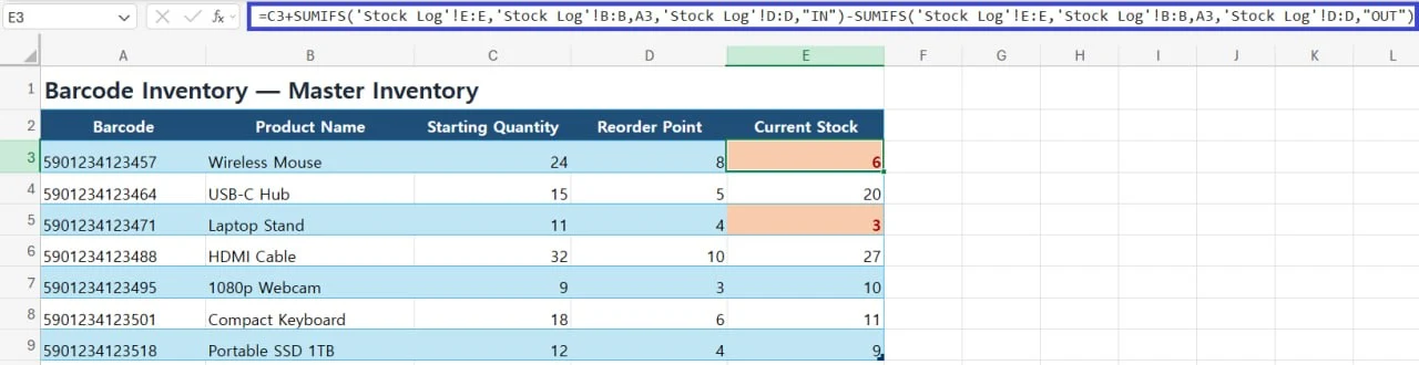
To flag low stock, select E3:E1002 — start at E3, the first data row — and go to Home > Conditional Formatting > New Rule > Use a formula to determine which cells to format. Enter:
=AND($E3<>"",$E3>=0,$E3<=$D3)
Pick a red fill. The rule flags stock at or below its reorder point, skips blank rows, and leaves negative balances for a separate rule.
Add that second rule now, with =AND($E3<>"",$E3<0) and a clearly different fill — amber works well. In this workflow, a negative on-hand balance is a data-quality exception, usually a duplicated OUT movement or a missing starting quantity. Because the low-stock rule explicitly excludes negative values, the two colors cannot compete, and a genuine data error never hides inside a sea of ordinary reorder flags.
If you also want movement history, select the Stock Log data and go to Insert > PivotTable: Barcode Scanned to Rows, Movement Type to Columns, Quantity to Values. The pivot shows flow per item; column E shows the balance. Because your timestamps are static, you can filter the source by date to build a clean monthly summary.
Expected outcome: A live on-hand count per product, with reorder candidates in red and impossible values in a second color.
The movement log keeps quantities current, but it does not independently prove that the shelf matches the workbook. Use our Excel inventory cycle count template to schedule blind counts, compare counted and system quantities, and route material variances through a recount workflow.
Step 6: Harden it before you hand it to staff
The workbook works at this point. It is not yet robust, and the gap shows up on day two rather than day one. Three small things cost about a minute each.
- Freeze the title and header rows. Select A3 — not the header row itself — then go to View > Freeze Panes > Freeze Panes. Everything above and left of the selected cell stays put, so rows 1 and 2 remain visible 400 rows into a scanning session. Freeze Top Row would pin only the sheet title in Row 1 and let your actual headers scroll away.
- Validate the Quantity column. Select E3 down on the Stock Log, then Data > Data Validation, whole number greater than 0, so nobody logs a movement of zero — or of “5 boxes”.
- Protect the Master Inventory tab and leave the Stock Log open. Staff need to add rows to the log; they never need to edit a product definition.
Expected outcome: A workbook that survives contact with a busy stockroom and a second pair of hands.
Common pitfalls and how to avoid them
- “Unknown Product” appears for a barcode that is definitely in your master sheet — or a code shows in scientific notation or loses a leading zero.
Cause: Excel is treating the identifier as a number in at least one of the two columns.XLOOKUPlooks for an exact match and a Text value never equals a Number value, so it never finds one. Separately, numeric entry removes leading zeros and values longer than 15 digits lose precision. The count is then wrong in a way that looks like a scanning problem rather than a formatting problem.
Fix: Format Master Inventory column A and Stock Log column B as Text before scanning. If data is already in, reformat and re-scan it — changing the format alone does not convert existing values or restore altered digits. - Every timestamp in the log suddenly shows the same time.
Cause: Someone used=IF(B3="","",NOW())because it looked convenient. NOW() is a volatile function: it recalculates whenever the workbook does, so every historical entry silently rewrites itself to the current time. Your audit trail is gone and nothing warned you.
Fix: Enter timestamps as static values —Ctrl+;, space,Ctrl+Shift+;. - A movement is logged but the count does not change.
Cause:SUMIFSmatches the literal strings “IN” and “OUT”. A typed “in ” with a trailing space, or “Out ” pasted from somewhere else, matches neither criterion, so the row is quietly excluded from both sums.
Fix: Force the values with a data validation dropdown on column D. If a count looks off, filter column D and check for anything that is not exactly IN or OUT. - The lookup returns the wrong product.
Cause: The same barcode appears more than once in Master Inventory, andXLOOKUPreturns the first matching result.
Fix: Highlight duplicate barcode values with Conditional Formatting, review the conflicting rows, and correct or delete the bad product record manually. Do not run Remove Duplicates blindly on the master database. - Current Stock goes negative.
Cause: In this workflow, a negative balance usually points to a duplicated OUT movement or a missing starting quantity. The formula is exposing a mismatch between the log and the physical count.
Fix: Add the=AND($E3<>"",$E3<0)conditional formatting rule from Step 5 so the exception surfaces in its own color instead of hiding among the reorder flags. - The scanner types unexpected characters.
Cause: In keyboard-emulation mode, the scanner and the operating system need compatible keyboard layouts. A mismatch maps scanned characters to the wrong keys, which is easy to misread as a faulty scanner.
Fix: Check the computer’s keyboard language first, then the scanner manual for its USB HID or Bluetooth HID country-keyboard setting.
When to adapt this workflow, and when to leave it
- Moving to Google Sheets. Worth it if the sheet needs to be reachable from more than one machine.
XLOOKUPandSUMIFScarry over unchanged. Google Sheets also supports data validation, conditional formatting, pivot tables, and frozen rows, but its menu paths differ from the desktop Excel steps above. The hardware remains the main practical difference: a USB scanner needs an OTG adapter to reach an Android tablet, and iPads generally work more easily with a Bluetooth scanner. If you stay in Sheets, low stock alerts in Google Sheets covers the reorder-threshold side in more depth. And if you go further than alerts, the same IN/OUT log convention powers our Google Sheets inventory dashboard build, which layers value, aging, and reconciliation views on top of the movement log. - Adding a second scanner. This is where the design stops holding. Excel and Google Sheets both support concurrent editing, but this workflow uses one shared Stock Log with no row reservation and no transaction lock, so two scan sessions can interleave records or compete for the same input area. Give each operator a separate log and consolidate afterwards, or move to software built for concurrent inventory transactions.
- Upgrading to dedicated software. Catalog size alone is a weak migration trigger. The stronger signals are structural: stock that must move when a sale closes, counts separated by location, or requirements for serial numbers, lot tracking, or shipping integrations. Those needs push beyond the simple shared-log design used here.
- Printing your own labels. For internal tracking, assign a unique item ID and encode it as Code 128. For products sold through retail or marketplace channels that require a GTIN, use a properly assigned GS1 identifier rather than inventing a UPC or EAN number.
What this setup costs
Most of the cost here is a one-time hardware purchase, not a subscription. US pricing checked July 2026.
| Item | Cost | Notes |
|---|---|---|
| Spreadsheet | $0 | Google Sheets and Excel for the web can both run the formulas; the menu paths and screenshots below follow desktop Excel. |
| Barcode scanner | Budget roughly $25–50 for a basic consumer scanner | Shopping prices vary by 1D/2D support, wired or wireless connectivity, and brand. Treat this as a starter budget, not a fixed market price. |
| Labels, if your products lack usable barcodes | Varies | Use existing product barcodes where possible. For internal IDs, price labels and printing separately based on label size, volume, and printer type. |
| Desktop Excel (optional) | $99.99/yr (Microsoft 365 Personal) or $249.99 one-time (Office Home & Business 2024) | Only if you want the desktop app. Home & Business is the perpetual edition that carries commercial-use rights; Office Home 2024 does not. If your team is already on Microsoft 365 Business Standard, that list price moved to $14 per user per month on annual commit effective 1 July 2026, with monthly commit priced higher; existing customers stay on their current price until renewal. |
Realistically, the new setup cost is mostly the scanner if you stay on Google Sheets or Excel for the web.
Comparing that against inventory software is not a hardware-payback calculation. A subscription is not buying you a scanner; it is buying you the things this workbook structurally cannot do — mobile scanning, several people updating at once, automatic stock movement on a sale, and location-level counts. The inventory spreadsheet vs. software guide works through where that line falls, and the Sortly setup guide shows what a barcode workflow looks like once it lives in an app instead of a workbook.
Download the workbook, or copy the formulas
If you would rather not build it from scratch, start from one of these:
- Blank template (.xlsx) — the two working tabs, headers, formulas, dropdowns, and both conditional formatting rules, ready for your catalog.
- Completed example (.xlsx) — seven products and thirteen logged movements showing how the master, log, and current stock formulas interact, plus a Movement Summary tab.
Four things about the downloads are worth knowing before you open them:
- Both files open on a Start Here tab that explains the workbook and repeats the Text-format and static-timestamp warnings. The two working tabs are the ones described above.
- Freeze panes, the IN/OUT dropdown, and the whole-number Quantity rule are already applied. Protecting the Master Inventory tab is left to you, because a locked template cannot be filled in.
- The workbook formulas use bounded ranges — rows 3 to 1002 — rather than the whole-column references shown in the steps above, so they can be pre-filled. That caps each sheet at 1,000 data rows. If you outgrow it, extend every range ending in 1002, including the conditional formatting range, or later rows are silently left out of the count.
- The files use
XLOOKUPthroughout, so the lookup columns return#NAME?on Excel 2016 and Excel 2019. The Start Here tab carries theVLOOKUPreplacement formula for those versions.
The completed example also includes a Movement Summary tab that totals IN, OUT, and net movement per barcode with formulas. It answers the same question as the PivotTable in Step 5 without rebuilding the pivot each time the log grows, so use whichever you find easier to maintain.
Or copy the formulas directly:
| Where it goes | Formula or setting |
|---|---|
| Master Inventory, column A | Barcode — format as Text before scanning |
| Master Inventory, E3 (fill down) | =IF(A3="","",C3+SUMIFS('Stock Log'!E:E,'Stock Log'!B:B,A3,'Stock Log'!D:D,"IN")-SUMIFS('Stock Log'!E:E,'Stock Log'!B:B,A3,'Stock Log'!D:D,"OUT")) |
| Conditional formatting on E3:E1002 — low stock | =AND($E3<>"",$E3>=0,$E3<=$D3) |
| Conditional formatting on E3:E1002 — impossible value | =AND($E3<>"",$E3<0) |
| Stock Log, column A | Static timestamp: Ctrl+; · space · Ctrl+Shift+; — never NOW() |
| Stock Log, column B | Scanned barcode — format as Text before scanning |
| Stock Log, C3 (fill down) | =IF(B3="", "", XLOOKUP(B3,'Master Inventory'!A:A,'Master Inventory'!B:B,"Unknown Product")) |
| Stock Log, C3 — Excel 2016 / 2019 | =IF(B3="", "", IFERROR(VLOOKUP(B3,'Master Inventory'!A:B,2,FALSE),"Unknown Product")) |
| Stock Log, column D | IN or OUT via a data validation dropdown, applied from D3 down |
| Stock Log, column E | Quantity — data validation, whole number greater than 0, applied from E3 down |
Sources and notes
Prices and product terms were checked in July 2026 against each vendor’s own pages.
- Microsoft — XLOOKUP function — syntax, the
if_not_foundargument, and confirmation that XLOOKUP is absent from Excel 2016 and Excel 2019. - Microsoft — NOW function — the volatile recalculation behavior behind the timestamp warning.
- Google Docs Editors Help — XLOOKUP — XLOOKUP support in Google Sheets.
- Microsoft 365 Personal — $99.99/year US pricing.
- Office Home & Business 2024 — $249.99 one-time price and commercial-use rights.
- Microsoft 365 pricing and packaging updates — the Business Standard price change effective 1 July 2026 and the renewal-timing rule.
- GS1 — Get a barcode / GTIN — the distinction between internal Code 128 labels and assigned GTIN, UPC, and EAN identifiers.
- Zebra — What is a 2D barcode? — the 1D versus 2D scanner distinction for QR codes.
Disclaimer
This guide is for general informational purposes only and does not constitute professional advice. Workflow steps, tool interfaces, feature availability, and pricing were verified against each product’s official documentation in July 2026 and may change without notice. The downloadable workbooks were built and checked by PickrTech; the sample rows in the completed example are fictional and should be replaced before use. Test any workflow on a copy of your data before relying on it.
Last reviewed: July 2026 by the PickrTech editorial team.