TL;DR: An inventory dashboard in Google Sheets needs four tabs — Items, Movements, Dashboard, and Checks — connected by SUMIFS, MAXIFS, and VLOOKUP formulas. This guide builds one on a 30-SKU sample dataset, so every number is checkable: 522 units on hand, $2,153.30 of inventory value, 3 SKUs at or below their reorder point, and 4 SKUs with no movement in 90+ days. You finish with five acceptance tests that prove the dashboard is reconciled against its source rows, all on a free Google account — and a free downloadable template with the full sample data included.

Before you begin: what you’ll need
You need a free Google account and a browser — nothing to install, and no paid add-ons. Have a basic list of your SKUs ready: product name, category, unit cost, current on-hand quantity, and a reorder point for each item. If you have not yet decided what fields, SKU codes, or reorder logic your inventory process needs, work through our vendor-neutral inventory management checklist first; this build assumes those decisions are already made.
Estimated time: 45–60 minutes for the core build. Difficulty: intermediate — you will write cross-tab formulas, but every formula is given in full. Cost: free.
The sample dataset behind every number in this guide
Generic dashboard tutorials show formulas but never numbers you can verify. This guide uses one fictional but fully worked dataset — a small home-goods store with 30 SKUs across four categories (Candles, Diffusers, Soaps, Accessories) and 48 stock movements logged between April and July 2026. All of the sample figures below come from that dataset, and the acceptance tests at the end reconcile against it. Here is an excerpt of the Items input data:
| SKU | Product Name | Category | Unit Cost | Starting Stock | Reorder Point |
|---|---|---|---|---|---|
| CAN-001 | Vanilla Soy Candle 8 oz | Candles | $5.40 | 30 | 10 |
| CAN-002 | Lavender Soy Candle 8 oz | Candles | $5.40 | 18 | 6 |
| DIF-003 | Ultrasonic Diffuser White | Diffusers | $14.00 | 10 | 5 |
| SOA-001 | Oatmeal Bar Soap | Soaps | $2.10 | 24 | 8 |
| SOA-008 | Goat Milk Bar Soap | Soaps | $2.60 | 10 | 4 |
| ACC-005 | Gift Box Small | Accessories | $0.90 | 40 | 10 |
And a few representative rows from the Movements log, which uses a strict sign convention — outgoing stock is negative, incoming stock is positive:
| Date | SKU | Movement Type | Quantity | Note |
|---|---|---|---|---|
| 2026-07-01 | CAN-001 | Sale | -4 | |
| 2026-07-11 | CAN-001 | Return | +1 | Customer return, resalable |
| 2026-07-15 | DIF-005 | Receipt | +12 | PO-1042 |
| 2026-07-18 | CAN-005 | Adjustment | -2 | Damaged in storage |
Headline totals for the sample, which we will rebuild step by step: 686 starting units, a net movement of −164 units, therefore 522 units currently on hand, worth $2,153.30 at unit cost. Every figure is an editorial calculation on this fictional dataset — it exists so you can verify that your formulas behave identically before trusting them with real stock.
Download: inventory-dashboard-google-sheets-template.xlsx — the complete workbook with a Read Me sheet and four working tabs, plus the 30-SKU sample data, formulas, validation dropdowns, conditional formatting, category chart, and reconciliation test. Upload it to Google Drive and save it as a native Google Sheet, or build the same system from scratch by following the steps below.
Step-by-step walkthrough
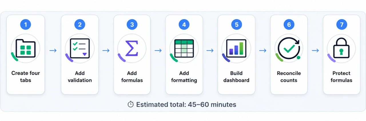
Step 1: Create the four-tab architecture
The reliability of a spreadsheet inventory system comes from strict separation of concerns. Create four tabs in a new Google Sheet: Items (one row per SKU — the master list), Movements (one row per stock change — the transaction log), Dashboard (calculated summaries only), and Checks (physical-count reconciliation).
In Items, set up columns A–F as inputs: SKU (A), Product Name (B), Category (C), Unit Cost (D), Starting Stock (E), and Reorder Point (F). Columns G onward will hold formulas you add in Step 3. Giving every SKU its own reorder point in column F is what lets the dashboard flag a slow $14.00 diffuser and a fast-moving bar of soap with the same rule.
In Movements, set up: Date (A), SKU (B), Movement Type (C), Quantity (D), and an optional Note (E). Use negative quantities for outgoing stock (sales) and positive for incoming (receipts, returns). This sign convention means current stock is always starting stock plus the sum of movements — no separate in/out columns to keep in sync. If you capture movements by scanning rather than typing, the same log structure powers our barcode scanner inventory workflow in Excel.
Expected result: a workbook where static product data and transactions never share a tab.
💡 Pro tip: format the SKU column as Plain text and the Date column as Date (Format > Number) so Sheets doesn’t auto-convert identifiers like “MAR-001” into dates.
Step 2: Configure data validation
In the Movements tab, select column C, then go to Data > Data validation and add a rule with the Dropdown criteria. Enter the four allowed values: Sale, Receipt, Return, Adjustment. Repeat in the Items tab for the Category column with your category names.
This matters more than it looks: a typo like “Acessories” silently splits a category into two, which later breaks both your dashboard chart and your SUMIFS category totals.
Expected result: movement types and categories can only be picked from a list, never typed freehand.
Step 3: Write the stock, value, and aging formulas
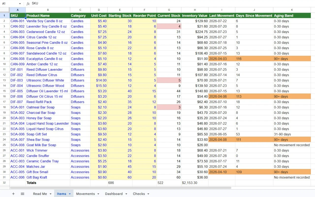
All calculated columns live in the Items tab, columns G–K. With 30 SKUs in rows 2–31, enter these in row 2 and fill down:
Current Stock (G2):
=E2+SUMIFS(Movements!$D:$D,Movements!$B:$B,$A2)
Inventory Value (H2):
=IF(ISNUMBER(G2),G2*D2,"")
Last Movement (I2):
=IF(COUNTIF(Movements!$B:$B,$A2)=0,"",MAXIFS(Movements!$A:$A,Movements!$B:$B,$A2))
Days Since Movement (J2): =IF($I2="","",TODAY()-$I2), and Aging Band (K2):
=IF($I2="","No movement recorded",IF($J2<=30,"0-30 days",IF($J2<=90,"31-90 days","90+ days")))
Check one SKU by hand before filling everything down. In the sample, CAN-001 starts at 30 and has three movements: a sale of −4 on July 1, a return of +1 on July 11, and a sale of −3 on July 22. So G should show 30 − 4 + 1 − 3 = 24, and H should show 24 × $5.40 = $129.60. If your formula returns 30, the SKU text in the two tabs doesn’t match exactly — usually a trailing space.
Note: the downloadable template ships these same formulas wrapped in blank-row guards — each begins =IF($A2="","",…) and uses bounded ranges like Movements!$D$2:$D$1000 — so an empty Items row can never distort a total or trigger a false flag.
Expected result: current stock, value, and aging update automatically every time a row is added to Movements.
Step 4: Flag stockout risk and aging with conditional formatting
Select G2:G31, open Format > Conditional formatting, choose “Custom formula is”, and enter:
=AND($A2<>"",$G2<=$F2)
with a red fill. Because the rule compares each row against its own column-F reorder point, no hardcoded threshold to maintain. Note the <=: in the sample, DIF-003 sits exactly at its reorder point (5 on hand, reorder at 5) and is correctly flagged — the boundary case you should test deliberately.
Add a second rule on I2:K31 with the custom formula =$K2="90+ days" and a yellow fill, so long-idle stock stands out. In the sample data, four SKUs last moved in early April 2026 (CAN-008, DIF-006, SOA-007, ACC-005), so by late July they all sit in the 90+ band; SOA-006 last moved on June 5 and lands in the 31–90 band.
This row-level flag tells you which items are at risk. If you want to go deeper on per-item reorder-point logic and alert options — including scripted email alerts — that is the job of our dedicated guide to low stock alerts in Google Sheets. This dashboard’s job, covered next, is summarizing risk across the whole inventory.
Expected result: with the sample data loaded, the Current Stock cell turns red on exactly three rows (CAN-002, DIF-003, SOA-001), and the aging columns turn yellow on the four SKUs in the 90+ band.
Step 5: Build the Dashboard tab with reconciled KPIs
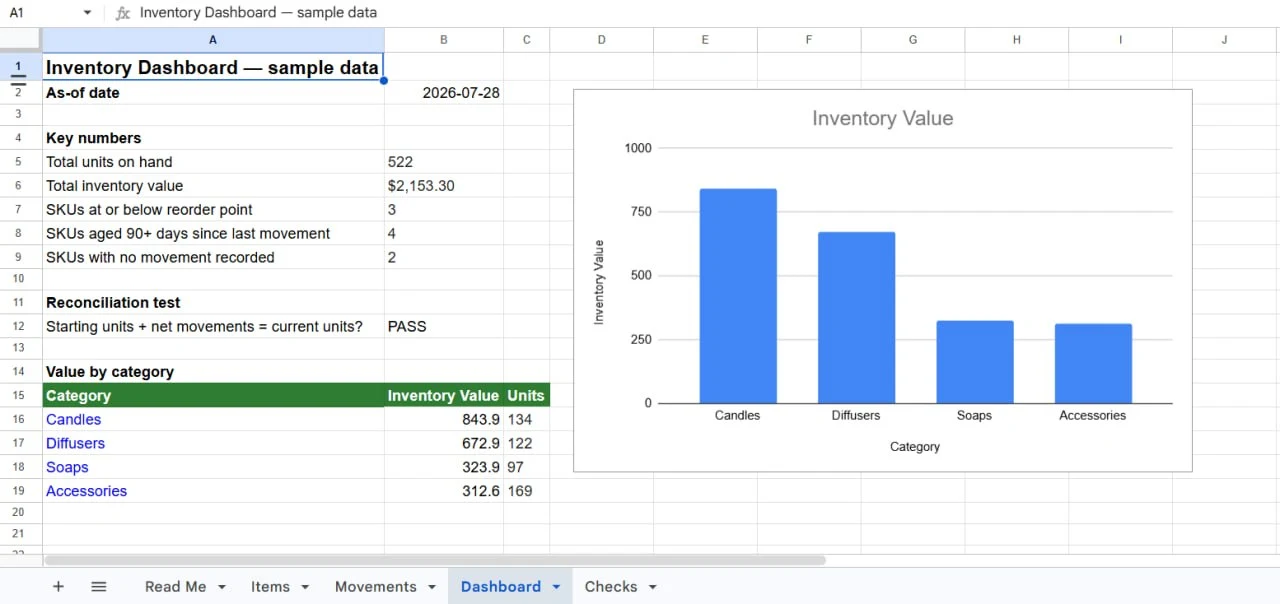
The Dashboard tab holds only formulas — never retyped numbers. Start with five key figures, shown here with the value each should return on the sample dataset:
| KPI | Formula | Sample result |
|---|---|---|
| Total units on hand | =SUM(Items!$G$2:$G$31) | 522 |
| Total inventory value | =SUM(Items!$H$2:$H$31) | $2,153.30 |
| SKUs at or below reorder point | =SUMPRODUCT((Items!$A$2:$A$31<>"")*(Items!$G$2:$G$31<=Items!$F$2:$F$31)) | 3 |
| SKUs aged 90+ days | =COUNTIF(Items!$K$2:$K$31,"90+ days") | 4 |
| SKUs with no movement recorded | =COUNTIF(Items!$K$2:$K$31,"No movement recorded") | 2 |
Below the KPIs, add the single most valuable cell in the whole workbook — a reconciliation test that proves the dashboard agrees with its source rows:
=IF(SUM(Items!$E$2:$E$31)+SUM(Movements!$D$2:$D$1000)=SUM(Items!$G$2:$G$31),"PASS","FAIL")
Starting units plus net movements must equal current units. On the sample: 686 + (−164) = 522, so the cell reads PASS. If it ever reads FAIL, someone has typed over a formula or entered a movement against a SKU that doesn’t exist — and you find out immediately, not at year-end.
Finally, build a small category summary — one row per category with =SUMIFS(Items!$H:$H,Items!$C:$C,$A16) for value and the same pattern on column G for units — then select it and use Insert > Chart to add a column chart. On the sample data the chart shows Candles $843.90, Diffusers $672.90, Soaps $323.90, Accessories $312.60.
Expected result: a Dashboard tab whose every number can be traced to a formula, with a live PASS/FAIL integrity cell.
Step 6: Reconcile physical counts in the Checks tab
The Checks tab is where cycle counts meet system data. Create columns: SKU (A), Counted Stock (B), System Stock (C), Variance (D), and Status (E). In C2:
=IFERROR(VLOOKUP($A2,Items!$A:$G,7,FALSE),"SKU not found")
The index is 7 because Current Stock is the seventh column of the A:G range — a common mistake is pointing VLOOKUP at Starting Stock instead, which makes every count look wrong. In D2 use =IF(ISNUMBER(C2),B2-C2,""), and in E2 =IF($D2="","",IF($D2=0,"OK","INVESTIGATE")), with a red conditional-formatting rule on any non-zero variance.
In the sample, a ten-SKU cycle count matches the system on nine items, but CAN-005 counts 12 against a system stock of 14 — variance −2, status INVESTIGATE. The correct fix is never to edit the Items tab: you investigate, and if the shrinkage is real, you log a −2 Adjustment row in Movements. The variance then closes to 0 on its own, and your history stays intact.
Expected result: discrepancies between shelf and system surface immediately, and every correction leaves an audit trail.
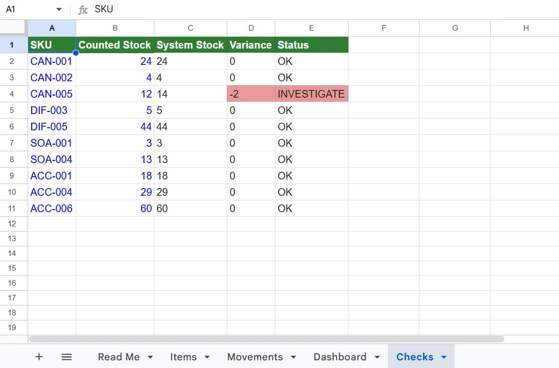
This Checks tab handles a basic physical-count reconciliation. For a recurring ABC schedule, blind count sheets, class-based recount tolerances, root-cause tracking, and monthly completion reporting, use our inventory cycle count template in Excel.
Step 7: Protect your formulas
Select the formula ranges — Items columns G–K and Checks columns C–E — then open Data > Protect sheets and ranges. Restrict editing to yourself while leaving the input ranges available to authorized editors.
Expected result: data entry stays open, formulas stay locked.
Acceptance tests: prove the dashboard before trusting it
Run these five tests before entering real data. With the sample dataset loaded, each has a known correct answer.
- Unit reconciliation. The Dashboard PASS/FAIL cell reads PASS, and the arithmetic checks by hand: 686 starting units − 164 net movement = 522 units on hand.
- Value reconciliation. Total inventory value equals the sum of the Items value column ($2,153.30), and one SKU verifies manually: CAN-001 is 24 × $5.40 = $129.60.
- Exception count matches the flags. Exactly 3 Current Stock cells are red in the Items tab (CAN-002, DIF-003, SOA-001) and the “SKUs at or below reorder point” KPI also reads 3 — including the boundary case DIF-003 at exactly its reorder point.
- Aging bands are correct. CAN-008 (last moved 2026-04-03) shows 90+ days; SOA-006 (2026-06-05) shows 31–90 days; SOA-008 and ACC-006, which have no movement rows, show “No movement recorded” rather than a false age.
- Checks tab closes the loop. CAN-005 shows variance −2 / INVESTIGATE. Add a −2 Adjustment row in Movements dated today; the variance recalculates to 0 and the unit-reconciliation cell still reads PASS.
If all five pass, clear only the sample input cells in Items columns A–F and the sample transaction rows in Movements. Do not delete entire Items rows or clear the formula columns G–K. The supplied template is prefilled for 30 SKUs; extend every related formula, KPI range, chart range, validation rule, and formatting rule together before adding a 31st SKU.
Setup mistakes to avoid
Typing manual stock counts. Never overwrite the Current Stock formula with a typed number. If you receive a shipment, log it as a new row in the Movements tab. Manual overwrites break your history and make every later reconciliation fail.
Using plain-text dates. If dates are stored as text, MAXIFS cannot compare them and your aging bands silently fail. Format date columns with Format > Number > Date.
Breaking data validation with copy-paste. Pasting rows from other spreadsheets can overwrite your dropdown rules. Paste with Ctrl+Shift+V (Cmd+Shift+V on Mac) to keep values only.
Ignoring SKU consistency. “SKU-001 ” with a trailing space is a different value from “SKU-001”. The SUMIFS match returns zero movements, and the item shows a false stockout. Test 1 above catches this — the reconciliation cell reads FAIL whenever a movement row references a SKU that isn’t in Items.
Common problems and fixes
#REF! or #VALUE! errors in SUMIFS formulas
⚠️ Cause: mismatched range sizes or a misspelled tab name. 🔧 Fix: if you sum Movements!D2:D500, the criteria range must cover the same rows (Movements!B2:B500) — or use whole-column references as in this guide, which cannot fall out of sync. Confirm the tab name in the formula matches the tab label exactly.
Stockout highlighting is not triggering
⚠️ Cause: the rule’s “Apply to range” doesn’t cover the row, or the custom formula’s row anchor is wrong. 🔧 Fix: the range must start at the same row as the formula references (range G2:G31 with a formula referring to row 2). Test with the boundary case: set one SKU’s current stock exactly equal to its reorder point — it must flag.
Dashboard chart shows blank or duplicate categories
⚠️ Cause: the chart range includes empty rows, or a typo split one category into two. 🔧 Fix: double-click the chart and tighten the data range to the summary table only, then confirm the Category column in Items uses the validation dropdown everywhere.
VLOOKUP returns #N/A or the wrong number in Checks
⚠️ Cause: #N/A means the counted SKU doesn’t exist in Items (usually a typo); a plausible-but-wrong number usually means the column index points at Starting Stock instead of Current Stock. 🔧 Fix: wrap the lookup in IFERROR as shown in Step 6, and make sure the index matches the position of Current Stock in your lookup range — 7 for Items!$A:$G.
When a spreadsheet stops being enough
This template is designed for a small, single-location workflow and is prefilled for 30 SKU rows. Google Sheets supports up to 10 million cells, but that technical ceiling is not a practical operating target. Consider dedicated inventory software when several locations need synchronized quantities, phone-camera scans must post stock changes immediately, or multiple operators need controlled transaction entry. Sheets can be extended with Forms, Apps Script, AppSheet, or add-ons, but those extensions introduce additional systems to configure, test, and maintain.
The decision about when workflow pressure justifies dedicated software has its own dedicated guide — inventory spreadsheet vs software: when to switch — and when you reach that point, our comparison of small business inventory management tools by free-plan limits covers what the move actually costs.
Frequently asked questions
Q: How do I handle product variants like sizes and colors?
A: Give each variant its own SKU row in Items so stock is counted precisely, and add a “Parent SKU” column if you want to group variants in a dashboard summary. Never track variants as one merged row — you lose the ability to flag which size is actually out of stock.
Q: Can data entry into Movements be automated?
A: Yes, but a linked Google Form writes responses to a form-response sheet; it does not automatically append clean rows to the existing Movements tab. Use that response sheet as the input log only when its columns and positive/negative quantity convention match this model, or map the responses into Movements with formulas or Apps Script. Test one receipt, one sale, and one invalid SKU before relying on the automation.
Sources and notes
All sample figures are editorial calculations on the fictional 30-SKU dataset described above. Technical behavior was checked against Google’s official documentation:
- SUMIFS function — Google Docs Editors Help — stock aggregation formulas
- MAXIFS — Google Docs Editors Help — last-movement-date formula
- VLOOKUP — Google Docs Editors Help — Checks-tab system-stock lookup
- Create an in-cell dropdown list — Google Docs Editors Help — data validation setup
- Use conditional formatting rules — Google Docs Editors Help — stockout and aging highlights
- Add & edit a chart or graph — Google Docs Editors Help — dashboard chart
- Protect, hide & edit sheets — Google Docs Editors Help — range protection
- Choose where to save form responses — Google Docs Editors Help — Google Forms response-destination behavior
- Files you can store in Google Drive — Google Drive Help — the 10-million-cell spreadsheet limit
Disclaimer
This guide is for general informational purposes only and does not constitute professional accounting, tax, legal, or financial advice. The dataset used throughout is fictional sample data created for demonstration; Google Sheets features and interface paths were checked against Google’s official documentation as of July 2026 and may change without notice. Always consult a qualified professional for advice specific to your business situation.
Last reviewed: July 2026 by the PickrTech editorial team.