TL;DR: A low stock alert in Google Sheets takes three things: a reorder point column, an IF formula that flags status, and a conditional formatting rule that colors the stock cell. Budget about 20 minutes. It costs $0 on a free personal Google account. It gives you a visual alert only; threshold-specific email alerts require Apps Script on a personal account, while eligible Google Workspace editions also offer built-in conditional notifications.
- Set reorder points from lead time and daily usage, not gut feel. The formula is only as good as the number behind it.
- Guard against blank rows, or every empty row in your formatted range will read “Reorder” in red.
- On a free personal Google account, threshold-specific email alerts require Apps Script. Google currently caps Apps Script at 100 email recipients per day for consumer accounts and 1,500 for Workspace accounts; eligible Workspace editions can instead use built-in conditional notifications.
- Sortly’s Free plan has no quantity alerts. Alerts begin on Advanced, listed at $49/month on monthly billing; annual and promotional pricing can differ.

The four checkpoints this guide walks through, from reorder points to the blank-row test
Who this setup fits — and who should skip it
This is for small business owners, solo operators, boutique retailers, and lean ops teams who already track physical inventory in a spreadsheet and keep getting caught by stockouts. You sell real products — online, in a shop, or out of a studio — and you want the sheet to tell you what to reorder instead of you scanning rows and guessing.
The setup below is deliberately small: five columns, one formula, two formatting rules. It is the fastest way to get a working reorder signal before you spend anything on software, and it stays useful even after you move on, because the reorder points you calculate here are the same numbers you will import into an inventory app later.
Skip it if you run multi-location warehousing with lot tracking, serialized inventory, or bin-level routing. Skip it if you need barcode scanning at receiving, purchase orders that flow into your accounting system, or stock levels that sync with a POS. Google Sheets does none of that, and bolting it on with scripts costs more time than a subscription does. If you want to stay in a spreadsheet but speed up counting, our barcode scanner with an Excel inventory spreadsheet guide covers the next practical setup.
There is also a people problem worth naming. A visual alert only fires if somebody keeps the numbers current. If your team already treats the spreadsheet as optional, coloring cells red will not fix that — the red cells will simply be wrong. Fix the counting habit first with a recurring inventory cycle count template in Excel, or move to a tool with mobile scanning so updating stock takes seconds instead of a laptop session.
What you need before you start
Tools
- A free Google account (a paid Google Workspace account is only needed if you later add email alerts at volume)
- Google Sheets
- Your product list, plus two numbers per item: how many you sell in a typical week, and how many days your supplier takes to deliver
People
- Lead operator: owns the file, sets reorder points, and is the only person allowed to touch the formula columns.
- Stock updaters (optional): anyone who counts. Give them spreadsheet Editor access, then protect the reorder-point and formula ranges under Data > Protect sheets and ranges so their working area is the Current Stock column and a stray paste cannot wipe out column E.
Estimated time: 20 minutes (10 to build, 10 to work out your first reorder points)
Difficulty: Beginner
Cost: $0
Build the alert in seven steps
Step 1: Set up your inventory columns
Open a new Google Sheet and put these headers in Row 1, columns A through E:
- A1: Item Name
- B1: SKU
- C1: Current Stock
- D1: Reorder Point
- E1: Status
Add three to five real items so you have something to test against. The screenshots in this guide use five, and you can copy them exactly if you want your sheet to match: Cotton T-Shirt (TEE-001), Canvas Tote Bag (BAG-002), Ceramic Mug (MUG-003), Linen Apron (APR-004), and Soy Candle (CAN-005). Put 15 in C2 and 20 in D2 for the T-shirt. Leave column E blank for now.
Before you go further, lock the number columns down. Select C2:D100, open Data > Data validation, add a rule, and set the criteria to a number greater than or equal to 0. Open Advanced options and confirm that invalid data is rejected rather than shown as a warning. The exact default can vary with an existing rule or imported sheet, so check the setting instead of assuming it. This prevents entries such as “out” or “n/a” from reaching the stock columns.
Expected outcome: A structured table where stock levels sit directly beside the thresholds they will be compared against, and where text cannot be entered into a number column.
Step 2: Set a reorder point that is actually right
Most spreadsheet alert systems fail here, not in the formulas. People pick a round number — 10, 50, 100 — and then wonder why the alert fires too late to be useful. A reorder point has one job: fire early enough that the replacement stock arrives before you hit zero.
The working version is:
Reorder point = (average units sold per day × supplier lead time in days) + safety stock
Say the Cotton T-Shirt sells 14 units a week, which is 2 a day, and your supplier takes 7 days from order to delivery. That is 14 units of demand during the lead time. Add safety stock — 6 units in this example, though a defensible buffer should reflect how much your demand and lead times actually vary — and the reorder point is 20. Now compare that with a round guess of 10: at 2 units a day, 10 units lasts 5 days against a 7-day delivery, so you sit empty for roughly two days on every reorder cycle.
Do this per item, not per catalog. In the example sheet the five items land on 20, 20, 20, 10, and 12 — the apron and the candle move slowly enough to justify a lower threshold. A slow-moving item with a local supplier might sit at 5. A fast seller shipped from overseas might sit at 300. If you want a more structured safety-stock estimate, Zoho publishes a free reorder point calculator that uses maximum daily usage, average daily usage, and lead time to calculate a buffer and reorder point.
Expected outcome: Column D holds a defensible number per SKU instead of a guess. Revisit these numbers quarterly, or whenever a supplier’s lead time changes.
Step 3: Calculate stock status with a formula
Click cell E2 and enter:
=IF(C2<=D2, "Reorder", "OK")
Press Enter. With 15 units against a reorder point of 20, the cell reads “Reorder”. Test the boundary while you are here: set C2 to 20 and it still reads “Reorder”, because the comparison is “at or below,” which is what you want. Set it to 21 and it flips to “OK”. Put it back to 15 before you continue.
To apply it down the list, click E2, grab the small blue square at the bottom-right of the cell (the fill handle), and drag to the last row of your data. Drag it only as far as your actual items go — see Step 5 for what happens if you drag it into empty rows.
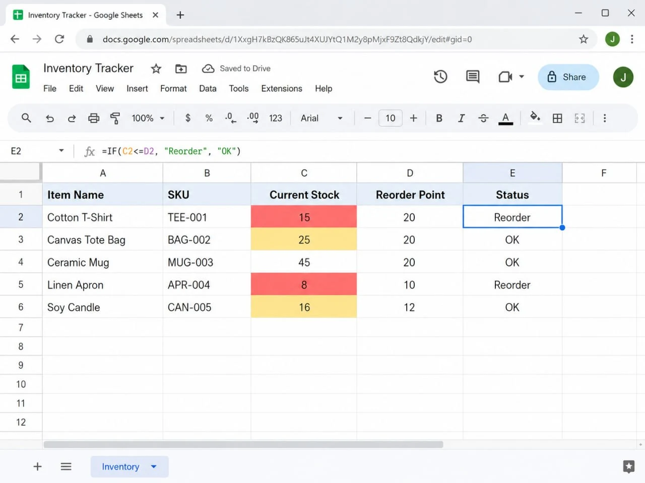
The IF formula in E2 compares current stock against the reorder point
Expected outcome: The Status column recalculates the instant anyone changes a stock count or a reorder point. No refresh, no rerun.
Step 4: Apply conditional formatting for the visual alert
Text in a Status column is easy to scroll past. Color is not. Set the Current Stock cell itself to turn red when it hits the threshold.
- Select the data range in Current Stock (for example, C2:C100).
- Go to Format > Conditional formatting.
- In the sidebar, change “Format cells if…” to Custom formula is.
- Enter:
=$C2<=$D2 - Set a red fill. Keep the text dark or white — whichever stays readable on your red.
- Click Done.
A note on the dollar signs, because most tutorials get this wrong. A custom formula is written for the top-left cell of the range and then applied relatively to every other cell in it. For a single-column range like C2:C100, =C2<=D2 works perfectly well — every cell in the range is already in column C, so nothing drifts. The locked form =$C2<=$D2 is what you want anyway, because it survives the two things you are likely to do next: widen the range across several columns to highlight the whole row, or copy the rule to another sheet. Google’s conditional formatting documentation has the full syntax.
Expected outcome: Any Current Stock cell at or below its own reorder point turns red the moment the number is entered.
Step 5: Stop blank rows from raising false alarms
Here is the trap almost every version of this tutorial walks into. You selected C2:C100 but you only stock five products. In a numeric comparison, Google Sheets evaluates an empty cell as zero — and zero is at or below every reorder point. Rows 7 through 100 all turn red, and the fill-handle drag from Step 3 stamps “Reorder” down 94 empty rows. Within a week nobody trusts the color anymore.
Two fixes, and you want both.
Guard the status formula. Replace the contents of E2 with this, then fill down:
=IF(OR(C2="", D2=""), "", IF(C2<=D2, "Reorder", "OK"))
Guard the formatting rule. Reopen Format > Conditional formatting, click your red rule, and change the custom formula to:
=AND($C2<>"", $D2<>"", $C2<=$D2)
Now an empty row stays empty and white. A genuine zero — an item that really is sold out — still turns red, which is exactly the distinction you need.
Expected outcome: Red means something. That is the whole point of the system.
Step 6: Add a yellow warning tier (optional)
Red means the item has already hit its reorder point: order now. A second tier flags items on the way there. A simple starting rule is 1.5× the reorder point — it is a visual buffer, not an inventory standard, and it does not convert to a fixed number of warning days.
- Select C2:C100 again and open Format > Conditional formatting.
- Click Add another rule and set it to Custom formula is.
- Enter:
=AND($C2<>"", $D2<>"", $C2>$D2, $C2<=$D2*1.5) - Set the fill to yellow and click Done.
- Check the order in the sidebar. The red rule must sit above the yellow one. Drag it up if it does not.
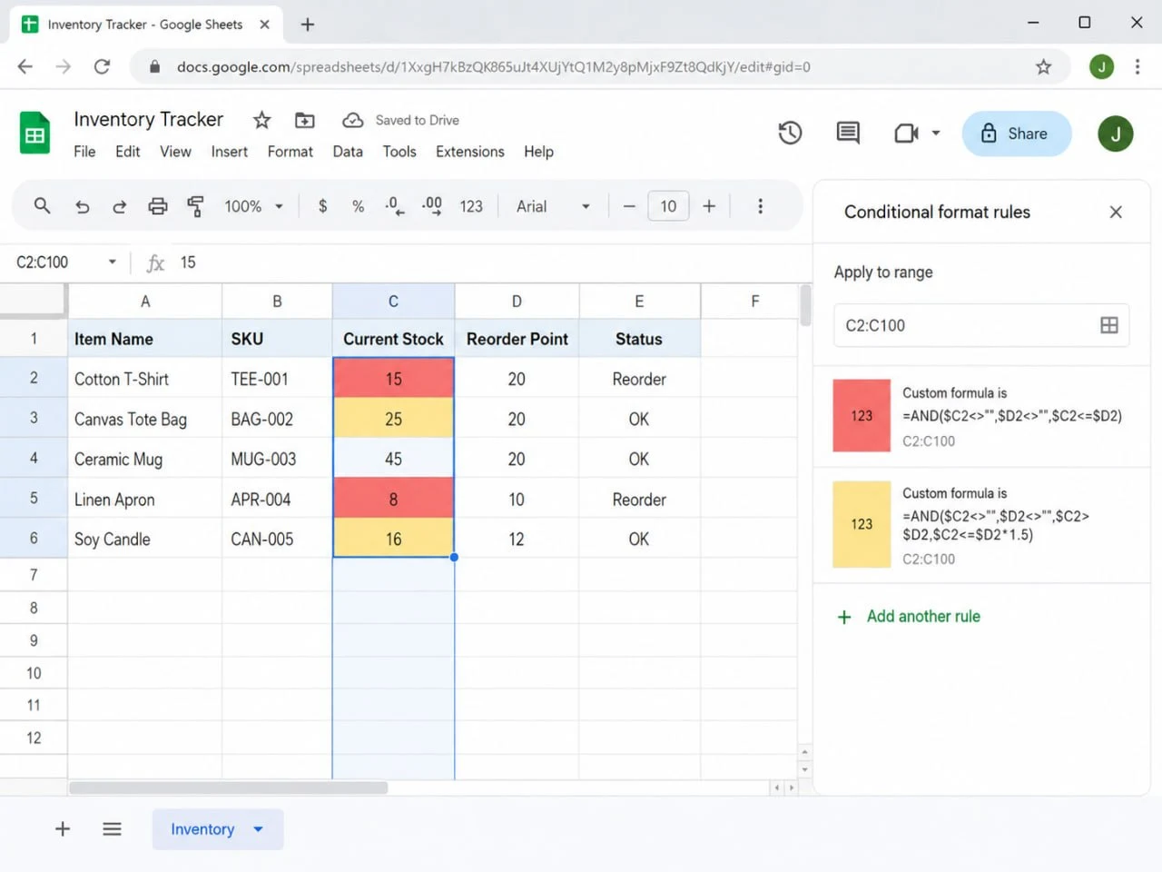
Both guarded rules in the Conditional format rules sidebar, red ordered above yellow, applied to C2:C100
The yellow rule includes $C2>$D2, so it only applies above the reorder point. That keeps the yellow and red conditions mutually exclusive: red covers stock at or below the reorder point, while yellow covers the buffer above it. Keeping the red rule above yellow still makes the rule list easier to audit, but the formulas no longer depend on priority to separate the two states.
Expected outcome: Three states at a glance — white (healthy), yellow (order soon), red (order now).
Step 7: Test it before you rely on it
Take the Cotton T-Shirt, sitting at 15 units with a reorder point of 20, and walk it through every state:
- Set Current Stock to
20. This is the boundary case: Status should read “Reorder” and the cell should be red, because the rule is “at or below.” - Set it to
25. Status flips to “OK”, but the cell should be yellow — 25 is above 20 and under 1.5 × 20 (30). - Set it to
35. The formatting clears. - Clear the cell entirely. Nothing should turn red, and Status should be blank.
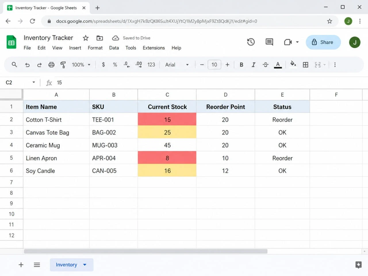
The finished sheet: two items below their reorder point in red, two inside the buffer in yellow, one healthy
The fourth check is the one people skip, and it is the one that catches a rule applied to the wrong range. If a color lands on rows you did not expect, open the sidebar and read the Apply to range field first — it often does not match the rows you meant to select. Run all four checks now rather than discovering the problem during a stockout.
Expected outcome: Every state behaves as designed. The sheet is now a reorder dashboard rather than a list.
Four things that break a Sheets low stock alert
- Blank rows show as “Reorder” in red. Why it bites: an empty cell can behave like zero in a numeric comparison, and a missing reorder point creates another false signal. Format C2:C100 with only five items in the sheet and the empty rows can light up or return misleading status values. Fix: use the guarded formulas from Step 5 —
=AND($C2<>"", $D2<>"", $C2<=$D2)for formatting and=IF(OR(C2="", D2=""), "", IF(C2<=D2, "Reorder", "OK"))for status. - Someone types “out of stock” into a number column. Why it bites: it does not throw a visible error. In a Sheets comparison, text ranks above any number, so
C2<=D2returns FALSE — the item quietly reads “OK” and never turns red, even though it is the one thing on the shelf you have run out of. Fix: apply the Step 1 validation rule (number ≥ 0) with Reject input switched on, and train the team to enter0, never words. - The yellow rule overlaps the red rule. Why it bites: a broad yellow condition such as
$C2<=$D2*1.5also matches items already at or below the reorder point. Fix: add$C2>$D2to the yellow formula so yellow only covers the buffer above the red threshold. Keep the red rule above yellow so the rule list is easy to audit. - The numbers are stale, so the colors are fiction. Why it bites: this is the failure mode that actually causes stockouts. A red cell built on a count from three weeks ago is worse than no alert, because you will act on it with confidence. Fix: add a “Last Counted” date column and put a recurring 10-minute count on the calendar. If the team cannot hold that habit, that is the signal to move to a tool with mobile scanning.
Adapting the workflow for tabs, notifications, and growth
- You track categories or locations on separate tabs. Build the alert on each tab, then create a Master tab and combine the item rows with
VSTACK. For example:=VSTACK(FILTER('Store A'!A2:E100,'Store A'!A2:A100<>""),FILTER('Store B'!A2:E100,'Store B'!A2:A100<>"")). Rebuild the conditional formatting rules on the Master tab because formulas bring across values, not formatting. UseIMPORTRANGEonly when the source data lives in a different spreadsheet file. Multi-location work is still the point where a spreadsheet starts fighting you — it is the workflow dedicated inventory tools are built around. - You want an actual notification. On a free personal Google account, a threshold-specific low-stock email requires Apps Script. A short script on a daily time-based trigger can scan the Status column and email you the list. Eligible Google Workspace editions also provide built-in conditional notifications for ranges that match a condition, so check Tools > Conditional notifications before writing code. If you use Apps Script, Google caps a consumer account at 100 email recipients per day and 90 minutes of total trigger runtime, against 1,500 recipients and 6 hours on a Workspace account. For one daily digest to yourself, either Apps Script quota is plenty, but you are now the developer and support team for that script.
- You want more than a per-row alert. The alert tells you which rows need action; a dashboard adds catalog-wide totals, inventory value, aging bands, and a reconciliation check on top. Our guide to building an inventory dashboard in Google Sheets shows the four-tab structure that produces those summaries.
- Your catalog is growing. The documented ceiling is 10 million cells per spreadsheet, far above the scale of this example, but that is a storage limit rather than a recommended operating target. Conditional formatting is re-evaluated as you type, and a heavily formatted shared file will feel sluggish in the browser long before any documented limit comes into play. Treat recurring lag, or counts that keep arriving late, as the practical signal to compare the trade-offs in the inventory spreadsheet vs. software guide.
The complete template and formulas
Copy this into Row 1 of a new sheet:
Item Name | SKU | Current Stock | Reorder Point | Status | Supplier | Unit Cost | Last Counted
Columns A through E are the five the alert needs. Supplier, Unit Cost, and Last Counted are optional additions that cost nothing to carry: Supplier tells you who to call when a row turns red, Unit Cost lets you total the value of what you are about to order, and Last Counted is the column that keeps the fourth pitfall above from quietly ruining the system.
| Where it goes | Formula |
|---|---|
| Status (E2, fill down) | =IF(OR(C2="", D2=""), "", IF(C2<=D2, "Reorder", "OK")) |
| Conditional formatting — red | =AND($C2<>"", $D2<>"", $C2<=$D2) |
| Conditional formatting — yellow | =AND($C2<>"", $D2<>"", $C2>$D2, $C2<=$D2*1.5) |
| Reorder point (D, calculate once per item) | (units sold per day × lead time in days) + safety stock |
Both formatting rules apply to the Current Stock range (C2:C100, or however far your data runs), with red ordered above yellow. If your data starts on a different row, change every 2 to your first data row.
How this workflow was tested
The sheet in the screenshots is a working Google Sheets file built for this guide, not a mockup: five items, the reorder points listed in Step 2, and both formatting rules applied to C2:C100. Every formula printed here was entered in that file and checked against the four failure modes that matter most in a small inventory sheet — blank rows inside the formatted range, non-numeric stock entries, a value sitting exactly on the reorder point, and a missing threshold.
Vendor plan names, caps, and prices were read in July 2026 from each vendor’s own pricing and help pages rather than third-party roundups. We did not run a hands-on trial of Sortly or Zoho Inventory for this guide; those details are documented plan boundaries, not tested behavior.
What this setup cannot do — and what to use instead
The honest limitation is the one in the TL;DR: this alert waits to be found. It costs nothing and it works, but nobody gets a push notification, and nobody scans a barcode. If either of those is the feature you actually need, a spreadsheet is the wrong shape of tool and no amount of formula work will fix it.
Free inventory apps can replace parts of this workflow, but the trade-offs differ. Sortly is the closest match when you want photo-based items, phone barcode scanning, and threshold notifications, but its Free plan covers 100 items and 1 user with no quantity alerts. Quantity alerts begin on Advanced, listed at $49/month on monthly billing, with 500 items and 2 users; annual and promotional pricing can differ. Zoho Inventory’s Free plan allows 50 orders a month, 1 user, and 1 location. It solves a different problem: it is an order and fulfillment system with sales-channel integrations rather than a drop-in replacement for this visual stock warning. For this five-column, zero-subscription alert, the spreadsheet remains the simpler option.
If this workflow has served its purpose and you are ready to move, the Sortly setup guide walks through the import and the barcode workflow — and the reorder points you calculated in Step 2 are the numbers you will import.
Sources and notes
- All vendor plan names, caps, and prices were checked in July 2026 against the vendors’ own pages.
- Google Docs Editors Help — Use conditional formatting rules in Google Sheets — custom formula syntax and rule prioritization.
- Google Drive Help — Files you can store in Google Drive — the 10 million cell ceiling per spreadsheet.
- Google for Developers — Quotas for Google Services — email recipient and trigger runtime limits for consumer vs. Workspace accounts.
- Sortly pricing page and Sortly Help Center — Quantity Alerts — plan prices, item and seat caps, and confirmation that alerts are excluded from the Free plan.
- Zoho Inventory pricing comparison — free and Standard plan order, user, and location limits.
Disclaimer
This guide is for general informational purposes only and does not constitute professional advice. Workflow steps, tool interfaces, plan names, and prices were verified against each product’s official documentation in July 2026 and may change without notice. Test any workflow on a copy of your data before relying on it.
Last reviewed: July 2026 by the PickrTech editorial team.